ON THE BACKWARD-IN-TIME PROBLEM IN POPULATION DYNAMICS

* This note is dedicated to my girlfriend KN…

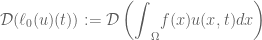
Starting from the open perspectives mentioned in the preprint as well as the note about the time-dependent backward-in-time parabolic problem in abstract form, we have successfully solved the nonlocal problem backward in time that arises in population dynamics by the quasi-reversibility (QR) method. One of the most important descriptions for the nonlocal effects can be easily followed by the local movement of species. In particular, from the biological and ecological aspects, the nonlocal term is provided in the diffusion by

$\mathcal{D}(\ell_{0}(u)(t)):= \mathcal{D}\left(\displaystyle{\int}_{\Omega} f(x)u(x,t)dx\right)$ .

The above expression contains $u$ that represents the population density of an individual species (we reduce ourselves to the single-species model due to the origin of the problem being considered), and the function $f$ mathematically describes the weight function that generalizes our analysis.

The need for the establishment of the nonlocal problem cannot avoid the density-related reaction term which represents the birth/death or the immigration/emigration in some certain cases. The structure of this nonlinear term is also very well known by the words: global Lipschitz and local Lipschitz. Notice that if one has the $L^{\infty}$ -bounds of the solution, the locally Lipschitzian can be reduced to the global one. That is the first point we would like to mention to facilitate the abyss in general. However, the underlying model we consider in this case has no requirement of that regularity, and that makes our contribution raw but greatly huge.

The backward-in-time problem is an inverse problem but totally different from the usual coefficients identification problem. In fact, the question is if we do know the information of the density at a certain time, say $T>0$ , how do we find the preceding data?

In principle, we have shortly revealed the expression of the following problem:

$\partial_{t} u - \mathcal{D}(\ell_{0}(u)(t))u_{xx} = \mathcal{R}(x,t,u),$

associated with the zero Neumann boundary condition which indicates the biological specimen is insulated. Last but not least, the final condition reads

$u(x,T) = g(x).$

For the sake of simplicity, we present the one-dimensional case, but in general the results can be extended to higher dimensions.

The main content is, at first, commenced by the absence of the reaction, i.e. $\mathcal{R}\equiv 0$ . In this case, we introduce a simple result (existence and uniqueness) as well as the representation of solution, then by the same token the solution for the backward case would be handled. Furthermore, we illuminate the jargon “ill-posedness” by showing a qualitative example in the sense that once the measurement noise $\varepsilon\in (0,1)$ that adheres to the final data tends to zero, the corresponding solution, denoted by $u^{\varepsilon}$ , cannot be computed by any numerical method. In this work, we prove that

$\displaystyle{\lim_{\varepsilon\to 0}} \left\Vert u^{\varepsilon} - u\right\Vert_{L^2} = \infty.$

The next flow can be recognized by considering the globally and locally Lipschitz cases of reaction. Employing the representation and under some assumptions on the parameters, we define the operator

$\Delta^{\varepsilon}[\cdot](t,x) := \displaystyle{\sum_{p\ge 1}} \lambda_{p}^{\varepsilon}\left\langle [\cdot](t),\phi_{p}\right\rangle \phi_{p}(x),$

which is expected to approximate the Laplace operator.

In the short-hand explanation, we have used above the eigenvalues and eigenbasis $\left(\lambda_{p},\phi_{p}\right)_{p\in \mathbb{N}}$ and the perturbed eigenvalues for this new operator, provided by

$\lambda_{p}^{\varepsilon} := -\dfrac{1}{{\eta}_{2}T}\ln\left( \beta + \mbox{exp}\left(-{\eta}_{2}T \lambda_{p}\right)\right),$

where $\eta_{2}>0$ denotes the upper bound of the diffusion and $\beta:=\beta(\varepsilon)\in (0,1)$ is the so-called regularization parameter.

This is the emphasis of this work if we do not mind a lot of techniques and computations, and the Sobolev spaces in combination with the Gevrey spaces used throughout the paper. Till the end, we prove that the error estimates, up to the locally Lipschitz case, are of order $\mathcal{O}({\beta}^{\frac{t}{T}})$ , which is also a confirmation to the error bounds of the original result in a monograph by Lattès and Lions since 1967.

As final words, although a huge mountain has been conquered, it is not the highest peak at all. The enlisted open perspectives in the work mentioned at the beginning of this note continue to remind us a lot of huge problems. Nobody knows which one could be done first, but let us aim ourselves at the contribution into the regularization theory of the system of equations which is more realistic and closely touches the applications.

This note is followed by the paper attached here. In the part of computational tools, we apply a symbolic-based computational method to obtain the algorithm. Also, we provide two numerical examples including the generalized KiSS model and the Fisher model to corroborate our analysis.

Vo Anh Khoa

The truest greatness lies in being kind, the truest wisdom in a happy mind